Polar maps
Seeing Polar Maps
Forecast relative to the night starting on 2026/06/15 MST
Note: click on a figure to magnify the image. Date of figures refers to the start of night in MST.
Horizontal maps average
Seeing Horizontal Maps Temporal Evolution
Forecast relative to the night starting on 2026/06/15 MST
Note: click on a figure to magnify the image. Date of figures refers to the start of night in MST.
Seeing horizontal map extended on a 50km x 50km square centred on LBT (represented with a black dot). The seeing is integrated over three different vertical slabs:
TOTAL SEEING (εTOT) – [dome-20000]m
BOUNDARY LAYER SEEING (εBL) – [dome-600]m
FREE ATMOSPHERE SEEING (εFA) – [600-20000]m
The seeing in each pixel is obtained integrating the CN2 along the zenith and covering the temporal range [dusk,dawn]. The black iso-lines represent the heights of the Digital Elevation Model (DEM).
εTOT AVERAGES:
Averages are computed over the whole night [<dusk> – <dawn>]UT and also in the first, central and last part of the night (see partition).

Fig 1: εTOT over the whole night [<dusk> – <dawn>] UT time frame
Fig 1: εTOT over the whole night [<dusk> – <dawn>] UT time frame

Fig. 2: εTOT over the “first part of the night”.

Fig. 3: εTOT over the “central part of the night”.

Fig. 4: εTOT over the “last part of the night”.
εBL AVERAGES:
Averages are computed over the whole night [<dusk> – <dawn>] UT and also in the first, central and last part of the night (see partition).

Fig. 5: εBL over the whole night [<dusk> – <dawn>] UT time frame
Fig. 5: εBL over the whole night [<dusk> – <dawn>] UT time frame
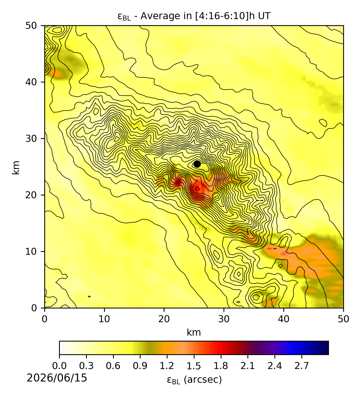
Fig. 6: εBL over the “first part of the night”.
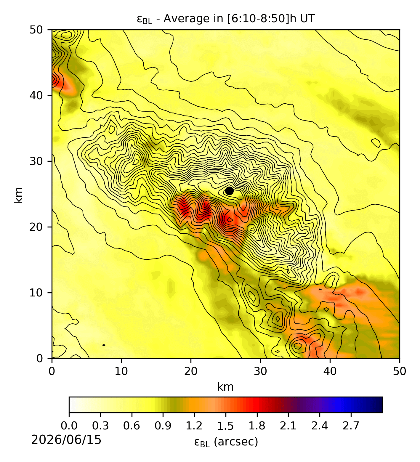
Fig. 7: εBL over the “central part of the night”.

Fig. 8: εBL over the “last part of the night”.
εFA AVERAGES:
Averages are computed over the whole night [<dusk> – <dawn>] UT and also in the first, central and last part of the night (see partition).

Fig. 9: εBL over the whole night [<dusk> – <dawn>] UT time frame
Fig. 9: εBL over the whole night [<dusk> – <dawn>] UT time frame

Fig. 10: εFA over the “first part of the night”.

Fig. 11: εFA over the “central part of the night”.

Fig. 12: εFA over the “last part of the night”.
Horizontal maps anim.
Seeing Horizontal Maps Temporal Evolution
Forecast relative to the night starting on 2026/06/15 MST
Note: click on a figure to magnify the image. Date of figures refers to the start of night in MST.
Seeing horizontal map extended on a 50km x 50km square surface centred on LBT (represented with a black dot). The seeing is integrated over three different vertical slabs:
TOTAL SEEING (εTOT) – [dome-20000]m
BOUNDARY LAYER SEEING (εBL) – [dome-600]m
FREE ATMOSPHERE SEEING (εFA) – [600-20000]m
The seeing in each pixel is obtained integrating the CN2 along the zenith and covering the temporal range [dusk,dawn]. The animations show the temporal evolution with 1-hour steps (in UT and MST). The black iso-lines represent the heights of the Digital Elevation Model (DEM).
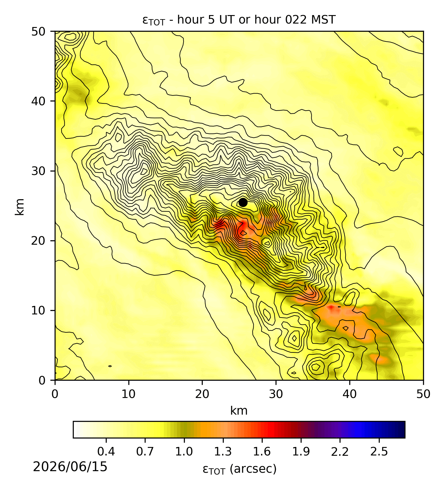
Fig. 1: Seeing map [50×50]km integrated on [20-20000]m. Time animation with 1-hour steps
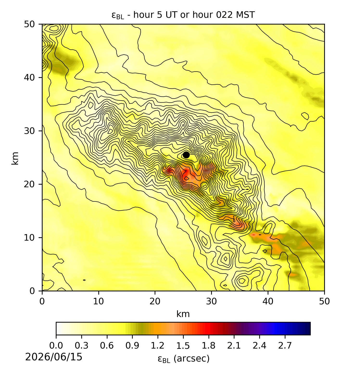
Fig. 2: Seeing map [50×50]km integrated on [20-600]m. Time animation with 1-hour steps

Fig. 3: Seeing map [50×50]km integrated on [600-20000]m. Time animation with 1-hour steps
Seeing Temporal Evolution
Seeing Temporal Evolution
Forecast relative to the night starting on 2026/06/15 MST
Note: click on a figure to magnify the image. Date of figures refers to the start of night in MST.
Temporal evolution of the seeing integrated in different vertical slabs between the sunset and the sunrise:
TOTAL SEEING (εTOT) – [dome-20000]m
BOUNDARY LAYER SEEING (εBL) – [dome-600]m
FREE ATMOSPHERE SEEING (εFA) – [600-20000]m
Astronomical dusk and dawn are shown too.
On the x-axis is time in UT (bottom), in MST (top). Mountain Standard Time MST=UT-7. Data points frequency is 2 minutes. Data points are re-sampled at a frequency of 20 minutes after a 1-hour moving average. The error bars are the sigma over the 20 minutes sampling, computed before the moving average.
For those cases in which there are in-situ real-time measurements, the website displays the following outputs:
- BLACK LINE: model forecast displayed at 14:00 MST.
- GREEN LINE: real-time measurements treated with a 1h moving average as the forecasts.
- RED LINE: short time scale forecasts computed each full hour and extended on the successive four hours.
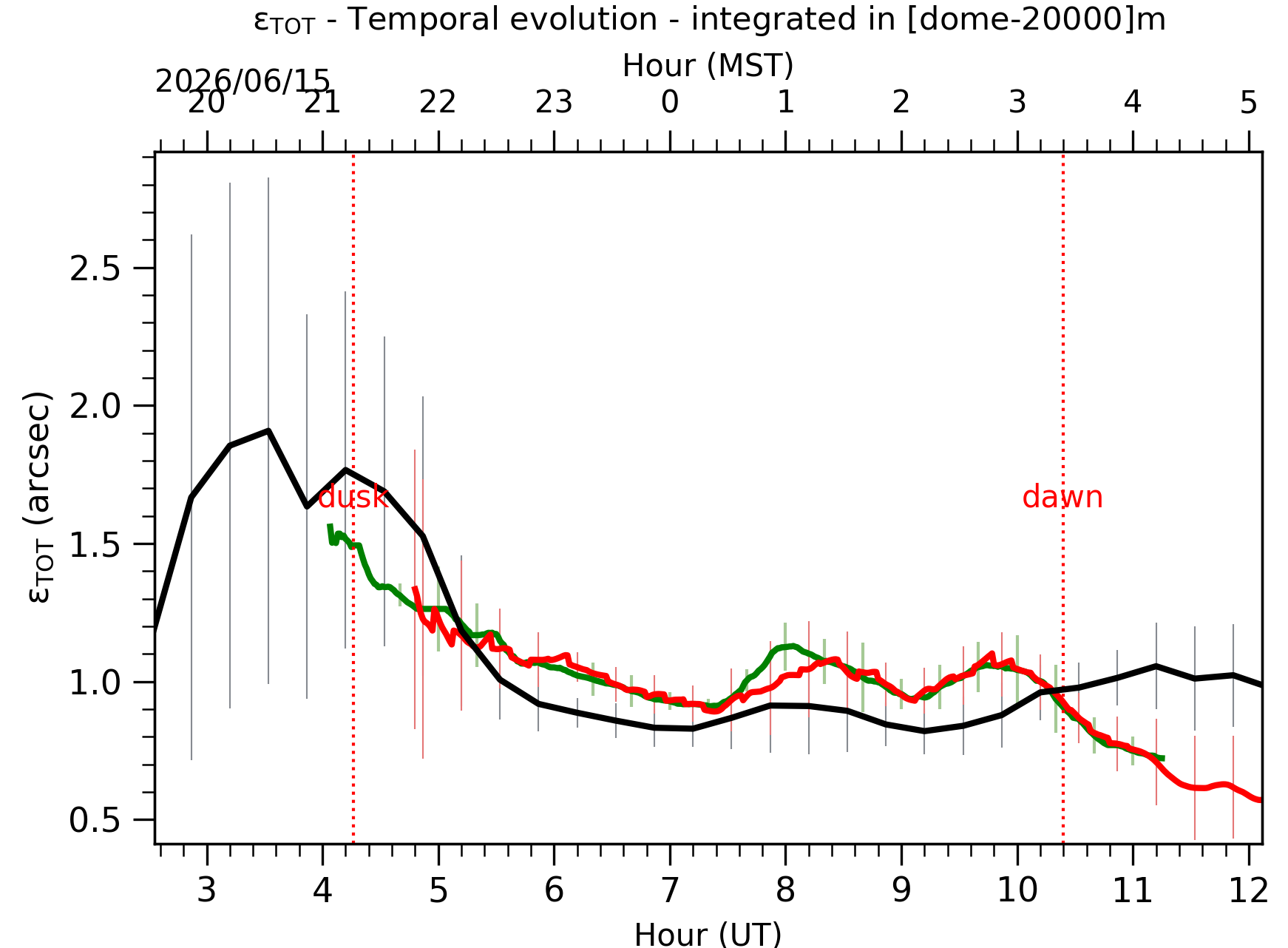
Fig. 1: Temporal evolution of εTOT ([dome-20km]) between the sunset and the sunrise.

Fig. 2: Temporal evolution of εBL ([dome-600m]) between the sunset and the sunrise.
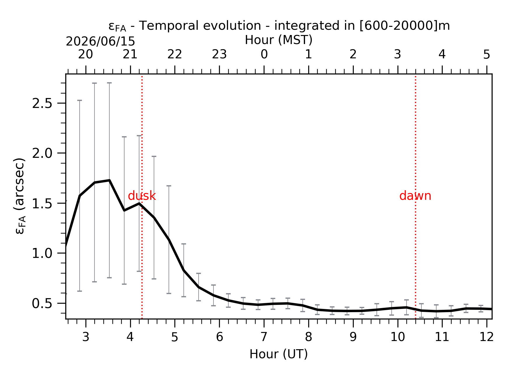
Fig. 3: Temporal evolution of εFA ([600m-20km]) between the sunset and the sunrise.